Janert - Feedback Control for Computer Systems [640b0277]

books, computers, control theory

1. Chapter 1 - Why Feedback

Sets up the book, motivates with reasons to establish control for queues
- interesting counterpart to queueing theory, where we'd traditionally model stuff as a feedforward system
Funny this book was written before Kubernetes, which was most people's introduction into a feedback system

2. Chapter 2 - Feedback Systems

Notes that you need to track amount of corrective action taken
Applying large control actions but need to avoid oscillatory behavior and kicking the system out of a stable state
states that the big 3 are: stability, performance, accuracy
- a lot is buried in accuracy though, since there's a tension between waiting the right amount of time for accurate data and being too slow to take corrective action (Spanner query retries, for example, sets a max wait time by waiting on epsilson)

3. Chapter 3 - System Dynamics

Contrasts lag with delay
Also mentions that computer systems can arbitrary change internal state, which is true but with a caveat
- Distributed systems tend to flow from known state to a known state, as multiple nodes typically need to coordinate to move states. A malfunctioning node just gets kicked out of the Paxos quorum, but the real disaster is SDC where multiple nodes agree on an invalid state.
  - Invariant checks are necessary for this, which also reduce the "arbitraryness" of computer programs
Forced response - pot heating up as the stove is turned on
Free response - the system returning to a natural state
Importance of lags and delays
- a lag is defined as a rounded, partial response
- a delay is a response with a wait time
He's mostly establishing the basis for hystersis loop
This chapter largely attempts to model what initiates and what knocks systems out of hystersis

4. Chapter 4 - Controllers

Finally getting to PID controllers
Makes the important point that open loops need to be much more complex than closed loops, as feedback is not immediate.
- Components in open loop systems, by default, tend to be more stateful, as they need to maintain internal memory
- Components in closed loop systems can afford to be stateless, as modified state is eventually flowed back somehow
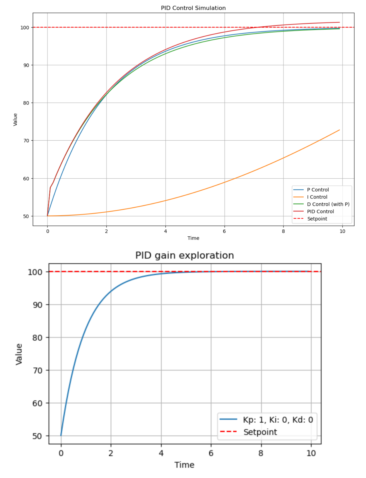
Porportional - we need to adjust our response in line with how far we've drifted, scalar
Integral - response must be adjusted to culumative error, which eliminates for steady state error
Derivative - improves overshoot, which responds to the rate of change in the error

  import matplotlib.pyplot as plt

  class PidController:
      def __init__(self, kp, ki, kd=0):
          self.kp, self.ki, self.kd = kp, ki, kd
          self.i = 0
          self.d = 0
          self.prev = 0

      def work(self, e, dt):
          self.i += dt * e
          self.d = (e - self.prev) / dt
          self.prev = e
          return self.kp * e + self.ki * self.i + self.kd * self.d

  def pid_simulation(setpoint, initial_value, kp, ki, kd, time_steps, dt):
      """Simulates PID control and returns the response."""
      controller = PidController(kp, ki, kd)
      value = initial_value
      values = [value]
      time = [0.0]  # Start time at 0.0

      for step in range(1, time_steps):
          error = setpoint - value
          output = controller.work(error, dt)
          value += output * 0.1  # Simulate plant response
          values.append(value)
          time.append(time[-1] + dt)

      return time, values

  # Simulation parameters
  setpoint = 100
  initial_value = 50
  time_steps = 100
  dt = 0.1  # Time step

  # P control
  time_p, values_p = pid_simulation(setpoint, initial_value, kp=0.5, ki=0, kd=0, time_steps=time_steps, dt=dt)

  # I control
  time_i, values_i = pid_simulation(setpoint, initial_value, kp=0, ki=0.01, kd=0, time_steps=time_steps, dt=dt)

  # D control (with some P to show damping)
  time_d, values_d = pid_simulation(setpoint, initial_value, kp=0.5, ki=0, kd=0.1, time_steps=time_steps, dt=dt)

  # PID control
  time_pid, values_pid = pid_simulation(setpoint, initial_value, kp=0.5, ki=0.01, kd=0.1, time_steps=time_steps, dt=dt)

  # Plotting
  plt.figure(figsize=(12, 8))

  plt.plot(time_p, values_p, label="P Control")
  plt.plot(time_i, values_i, label="I Control")
  plt.plot(time_d, values_d, label="D Control (with P)")
  plt.plot(time_pid, values_pid, label="PID Control")
  plt.axhline(y=setpoint, color='r', linestyle='--', label="Setpoint")
  plt.xlabel("Time")
  plt.ylabel("Value")
  plt.title("PID Control Simulation")
  plt.legend()
  plt.grid(True)
  plt.show()

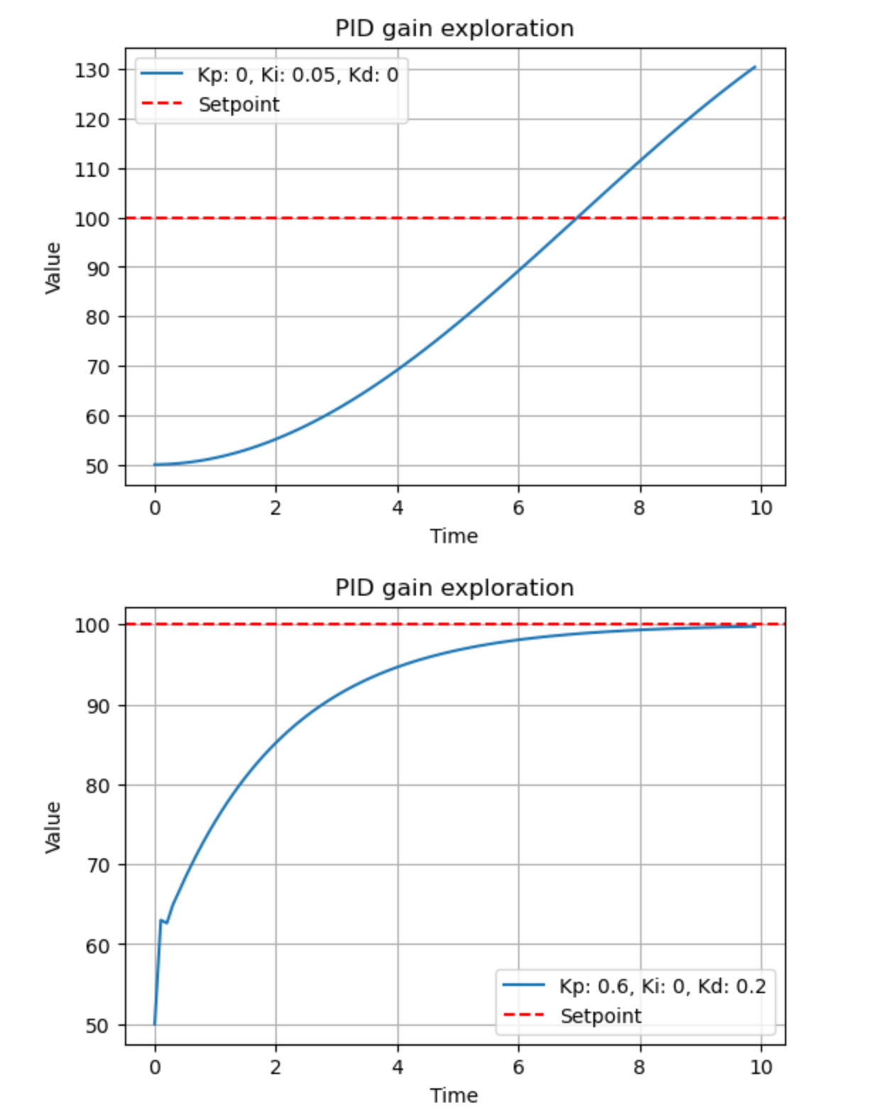
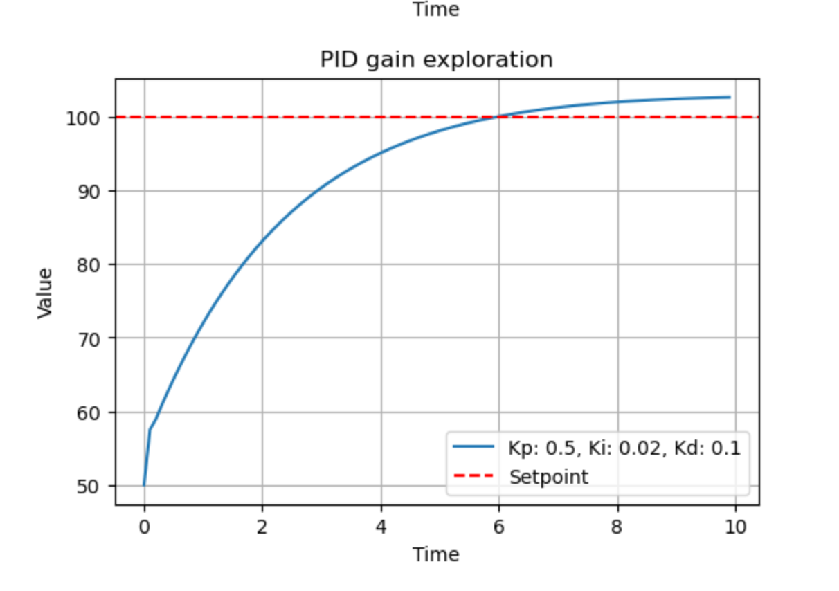
  def explore_gain(kp, ki, kd):
      time, values = pid_simulation(setpoint, initial_value, kp, ki, kd, time_steps, dt)
      plt.figure(figsize=(6,4))
      plt.plot(time, values, label = f"Kp: {kp}, Ki: {ki}, Kd: {kd}")
      plt.axhline(y=setpoint, color = 'r', linestyle = '--', label = "Setpoint")
      plt.xlabel('Time')
      plt.ylabel('Value')
      plt.title('PID gain exploration')
      plt.legend()
      plt.grid(True)
      plt.show()

  #Example of exploring gains.
  explore_gain(1, 0, 0)
  explore_gain(0, 0.05, 0)
  explore_gain(0.6, 0, 0.2)
  explore_gain(0.5, 0.02, 0.1)

Keyboard shortcuts